|
This is a burp of an idea. The roughness of the post reflects the lack of manners of the belch.
So there's this paper that I think is really important. It's new, but it consolidates some old points in a beautiful demonstration: https://arxiv.org/abs/1906.09012 Roads&Love demonstrate that the statistical distributions of concepts as they're elicited from text (amodal sources) are well-matched by the statistical distributions of concepts as they're elicited from perceptual sources (their demonstration used visual stimuli). Okay lame and boring, what does it mean. I think this paper has huge and broad implications regarding communication and meaningful interaction. Insofar as communication requires the conceptual alignment of multiple agents, this paper implies that communication is actually possible between two agents. Okay, why is it valuable to demonstrate that communication (here, I mean the conceptual alignment of multiple agents) is actually possible. Isn't it obvious that communication is possible (here, I would cite and recite Quine and Putnam). The answer from philosophers would be no, it isn't self evident that multiple agents can align their conceptual systems such that communication is possible. Hence the value of an empirical demonstration. But more importantly, this study illuminates the constraints by which such an alignment could occur. Namely, two amodal conceptual systems could align insofar as they're based on the same underlying system of concepts. The fact that Roads&Love could align an amodal text-based system of concepts and a perceptual image-based system of concepts is due to the fact that the text upon which the amodal system of concepts is based emerges from language use that emerges from perception. The development of text is inherently grounded in perception, and therefore the two systems can be aligned. Extending this to communication, the extent two which two agents' conceptual systems are grounded in the same subset of reality (assuming that reality is the thing that is sampled for the construction of conceptual systems) determines the extent to which these systems can align, and thereby the extent to which communication can occur. What are the constraints of communication? A shared set of perceptual experiences - in order for communication to happen between agents, a conceptual system grounded in the same set of perceptual experiences is necessary. Between agents of the same kind (e.g. humans), the majority of the work is carried by the perceptual systems being nearly identical - identical perceptual systems means that the agents have access to the same subset of reality as one another. Perceptual systems that are too highly varied may yield perceptually based concept systems that are not easily aligned. But even with shared perceptual systems, the experiences accrued by an agent may be such that the yielded conceptual systems of that agent may not be well-aligned to another agent. La vie. But moreover, since the most interesting this is the conceptual alignment between agents that can communicate, we need to talk about the conceptual systems that emerge from amodal sources, such as language or text. (Language serves as a means of sharing conceptual systems) If the amodal conceptual systems between two agents are not well-aligned, it might be for two (or more?) reasons. First, it might be because the perceptual experiences accrued by the agents from which the linguistic conveyance of amodal conceptual systems are derived are thoroughly dissimilar (can communication happen in this case? it's hard to say); in this case, even though linguistic inputs are well-aligned to perceptual experiences, conceptual alignment becomes challenging. Second, it might be that, even though the perceptual experiences of the agents are aligned, the construction of the linguistic inputs for one or both of the agents emerge from a different statistical distribution than that which is accessible from perception (honestly, I think this is an interesting case, and potentially a source of ought). So then, how do we increase the degree to which communication can occur between agents? If shared perceptual experiences generate conceptual systems that can be aligned, then as shared experiences between agents increases, the degree of possible communication between agents increases (likewise, as shared perceptual experiences decrease, the ability for agents to communicate decreases). But this is dependent on the degree to which the amodal conceptual systems align, since communication occurs through amodal avenues. If amodal conceptual systems emerge along a statistical structure that do not align with the statistical structure of that which can be perceived, then the potential of communication occurring decreases, since the conceptual systems cannot be aligned. This is really a pedantic way of saying that communication requires shared experiences, mediated by overlapping ideologies. But it provides a framework where these constructs can be formalized and empirically tested This makes a large claim about the degree to which communication can occur based on conceptual alignment. Can empirically test this. Find conceptual alignment of participants using like a similarity rating task for items in a particular domain (politics and religion are salient, could also do scientific topics, or other domains of expertise). Similarity rating task yields the conceptual system for a particular participant. Pair off participants and have them discuss topics within a particular domain for some alotment of time (10 minutes?). After discussion, have participants do an exit survey. Ask questions about how well they understood the other person's perspective, how well they conveyed their ideas, how well the other person understood what they said, whether they had to dumb down or hold back while discussing their position (did they hold back because they thought the other person wouldn't get it?)
5 Comments
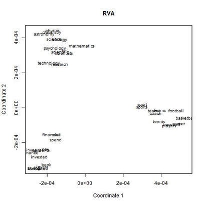
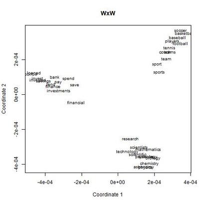
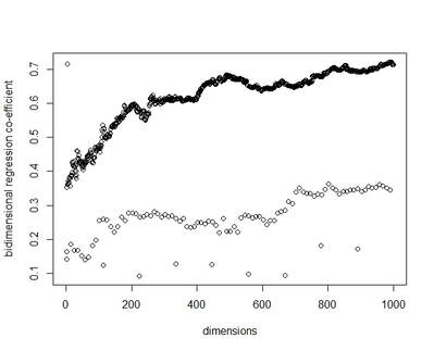
I recently wrote some code for a random vector accumulator. It worked pretty fast. But the reason it worked fast was because it was just a matrix multiplication between a word-by-word matrix and a matrix of random vectors. Upon reflection, I came to the frustrating conclusion: A random vector accumulator doesn't do anything that a word-by-word co-occurrence matrix doesn't do. Specifically: if the random vectors are defined as having a length of one, and a cosine similarity of zero with any other vector, then a sparse vector where only one element is one and the rest of the elements are zero fulfills this requirement. In this way, a count matrix can be construed as a special case of the random vector accumulator. Additionally, the random vectors add no information in addition to a word-by-word count matrix. Below are two MDS renderings of a given word list. First is the rendering for the RVA, the second is the rendering for the WxW matrix. The bidimensional regression yields an r value of 0.996, quantitatively demonstrating that the two renderings are a near-perfect match (only near-perfect because of the small amount of noise from the random vectors).  MDS projection of a selection of words (used in Jones & Mewhort, 2007). The words are drawn from three clusters in order to demonstrate the model's ability to correctly group similar words. The random vectors have 1000 elements/dimensions.  The word by word matrix is a raw frequency count of words that co-occur in the same context. Context is arbitrarily defined - here it's the co-occurrence of words within a paragraph. Upon further reflection (after it was pointed out to me), I realized that the nearly perfect reproduction of the WxW matrix by the RVA is a feature rather than a bug. While the RVA doesn't serve to reveal any latent relationships between words, it effectively compresses the matrices. The WxW matrix is ~95,000x95,000. The RVA matrix is ~95,000x1000, effectively (and with high accuracy) reducing the matrix to one one-hundredth of the size. (In practice, I used a scipy.sparse.csr_matrix to implement the count matrix - storing a 95,000x95,000 matrix in my computer's memory would be a mission; additionally, the transformation from a WxW matrix to an RVA is a simple matrix multiply between two matrices. The computation is sped up if I only use the words of interest from the WxW document. In this example, it was a matrix multiplication of my W'xW matrix [35,95000] and my random vectors [95000,1000] - which is a pretty quick computation. I've posted the code here.) In order to satiate my interest in RVAs, I looked at the ability of an RVA to reproduce the distributions of a random set of 1000 words at varying dimensionalities.  The x-axis is the varying number of dimensions. The y-axis is the bidimensional regression co-efficient (Friedman & Kohler, 2003; bidimensional regression is a measure of how well two plots match each other, independent of flips or rotations) Note that the RVA performance peaks at 0.7 rather than 1 (as in the above example). This is due to an interaction of the word set and the bidimensional regression measure. Plots that are well-clustered are generally easier to reproduce. Since I chose random points, any reproduction of the plot is going to be much noisier (I don't have a mathematical explanation for this, it's based on intuition earned from another project regarding spatial layouts; potentially forthcoming as a blog post).
There are a couple interesting points to note about this plot. First, there is a roughly linear increase in performance with dimensionality. This is to be expected. But there's this weird harmonic looking thing happening, where at certain intervals, the model drops in performance. I don't have any explanation for this (but I ran it multiple times to the same effect). It's neat, but weird. In final consideration, using a sparse matrix may still be more efficient. With a sparse matrix, I may have to store fewer actual elements than if I store a random vector. Potentially, instead of a random vector, there could be optimal vectors that I could use to reduce dimensionality while also reducing the actual number of elements that have to be stored. Or just a convenient plot device?She kinda seems like a Ravenclaw to me.¶I was playing around with the Harry Potter books (for a post that is yet to be released), when the realization hit me: I could use the computational power of semantic models to figure out whether Hermione really belongs to Gryffindor, or if she's actually a Ravenclaw. Here's a rough outline of the process.
Note:¶Click the button below to hide/show the raw code
In [1]:
from IPython.display import HTML

HTML('''<script>
code_show=true;
function code_toggle() {
 if (code_show){
 $('div.input').hide();
 } else {
 $('div.input').show();
 }
 code_show = !code_show
}
$( document ).ready(code_toggle);
</script>
<form action="javascript:code_toggle()"><input type="submit" value="Hide/Show the code."></form>''')
Out[1]:
In [5]:
import nltk
import numpy as np
import matplotlib.pyplot as plt
import matplotlib.axes as axes
from itertools import compress
import pickle
from scipy import sparse
from scipy.sparse.linalg import svds as svd
In [ ]:
# load file
def read_file(nums):
    text = ''
    for num in nums:
        with open('../../../corpus/HarryPotter/text/hp' + str(num) + '.txt', 'rt',encoding='utf-8') as file:
            for line in file:
                text = text + line
    return text

# read in a file
book_content = read_file(range(1,8))

# load character names and houses
with open('character_words.p', 'rb') as file:
    character_words = pickle.load(file)
In [ ]:
# tokenize on word
tokenized = nltk.word_tokenize(book_content)

#lowercase each word
tokenized_lower = [i.lower() for i in tokenized]
In [ ]:
frequencies = nltk.FreqDist(tokenized_lower)
Reducing the corpus¶Here's a plot showing the 5000 most frequent words used in Harry Potter. The shape of the curve is an inverse exponential, commonly referred to as a Zipfian Distribution. Simply put, most words don't occur that commonly, but the frequencies of a few words vastly outweighs that of the rest. These words (referred to as stop words) are removed from a corpus - their overwhelming frequency often prevent semantic models to pick up on any meaningful associations between words.
In [226]:
y = list(zip(*frequencies.most_common()))[1][:5000]
x = np.arange(1,len(y) + 1)
plt.plot(x,y)
plt.ylim([0,4000])
plt.axvline(200, color = 'red')
plt.show()
In [ ]:
# find the 50 most common words from the corpus
most_common_words = list(zip(*frequencies.most_common(200)))[0]

# keep character names though
most_common_words = list(set(most_common_words) - character_words)
In [ ]:
# find the words that only occur once
words,freqs = list(zip(*frequencies.most_common()))
least_common_words = list(compress(words, [bool(i <= 5) for i in freqs]))
In [ ]:
# remove most and least common words from the corpus
stop_listed_text = [i for i in tokenized_lower if (i not in most_common_words) & (i not in least_common_words)]
In [220]:
print('Length of original corpus: ' + str(len(tokenized_lower)))
print('Length of reduced corpus: ' + str(len(stop_listed_text)))
print(str(np.round((1 - len(stop_listed_text) / len(tokenized_lower)) * 100, 2)) + '% reduction')
Length of original corpus: 1392955
Length of reduced corpus: 447443
67.88% reduction
In [ ]:
with open('stop_listed_text.p', 'wb') as file:
    pickle.dump(stop_listed_text, file)
In [6]:
with open('stop_listed_text.p', 'rb') as file:
    stop_listed_text = pickle.load(file)
In [7]:
# make a scrolling window - width=4 words
# we're going to do a tapered window
windowed_text = []
length_window = 10
for i in np.arange(len(stop_listed_text) - length_window):
    windowed_text.extend(stop_listed_text[i:i + length_window])
In [8]:
# make a dictionary
words = sorted(list(set(stop_listed_text)))
dictionary = dict(zip(words, np.arange(len(words))))
In [9]:
# convert text to a word by document matrix
data = 1 - np.arange(0,1,1/length_window)
data = np.tile(data, len(stop_listed_text) - length_window)

rows = np.arange(len(stop_listed_text) - length_window)
rows = np.repeat(rows, length_window)

cols = [dictionary[word] for word in windowed_text]

wd = sparse.csr_matrix((data, (rows, cols)), shape=(len(stop_listed_text) - length_window, len(dictionary)))
In [25]:
# reconstruct matrix along word and reduced document dimensions
# get ww
ww = np.dot(wd.transpose(),wd).tolil()

ww = np.array(ww.transpose() / wd.sum(0)).transpose()
#save this
# with open('ww_hp.p','wb') as file:
#     pickle.dump(ww,file)
In [26]:
# for each house name and each character name, set all house and character names to 0
with open('character_words.p','rb') as file:
    character_words = pickle.load(file)
house_character_names = list(set(words).intersection(character_words))

for i in house_character_names:
    for j in house_character_names:
        ww[dictionary[i],dictionary[j]] = 0
In [27]:
def cosineTable(vects):
    return np.dot(vects,vects.transpose()) / np.outer(np.sqrt(np.sum(vects*vects,1)),np.sqrt(np.sum(vects*vects,1)))
What did we find out?
In [30]:
names = ['ravenclaw',
        'gryffindor',
        'hufflepuff',
        'slytherin',
        'harry',
        'cho',
        'cedric',
        'draco',
        'justin']

rows = [dictionary[i] for i in names]
test = ww[rows]
values = cosineTable(test)[:4,4:]
In [31]:
labels = names[4:]
ravenclaw = values[0]
gryffindor = values[1]
hufflepuff = values[2]
slytherin = values[3]

x = np.arange(len(labels))  # the label locations
width = 0.35  # the width of the bars

fig, ax = plt.subplots()
ax.bar(x - (width/4 * 2), gryffindor, width, label='Gryffindor',color='#ae0001')
ax.bar(x - (width/4 * 1), ravenclaw, width, label='Ravenclaw', color='#033e8c')
ax.bar(x + (width/4 * 1), hufflepuff, width, label='Hufflepuff',color='#ffdb00')
ax.bar(x + (width/4 * 2), slytherin, width, label='Slytherin',color='#2c8309')

# Add some text for labels, title and custom x-axis tick labels, etc.
ax.set_ylabel('Characters')
ax.set_title('Similarity between House and Character')
ax.set_xticks(x)
ax.set_xticklabels(labels)
ax.legend()

fig.tight_layout()

plt.show()
The figure above plots the similarities between the vectors representing each character and each house. The x-axis is the character, the y-axis is the cosine similarity (you'd better be impressed by the colors - I scoured the internet for the best hex-codes). I wanted to make sure that the model could correctly place a character in each house - Harry (obviously) has to be placed in Gryffindor, I chose Cho Chang to represent Ravenclaw, Draco to represent Slytherin, and Cedric Diggory to represent Hufflepuff. I was a little annoyed that the model placed him in Gryffindor (I guess he wasn't that great of a finder after all), so I had to dig deeper to find another Hufflepuff to validate my model. I settled on Justin FinchFletchley as representative (oh come on, you know who he is.. he's the one who did the one thing that one time...). Anyway, the model can correctly identify the houses for representatives for each house. With the model modestly validated, let's see how it sorts Hermione:
In [32]:
names = ['ravenclaw',
        'gryffindor',
        'hufflepuff',
        'slytherin',
        'hermione']

rows = [dictionary[i] for i in names]
test = ww[rows]
values = cosineTable(test)[:4,4:]
In [33]:
labels = names[4:]
ravenclaw = values[0]
gryffindor = values[1]
hufflepuff = values[2]
slytherin = values[3]

x = np.arange(len(labels))  # the label locations
width = 0.35  # the width of the bars

fig, ax = plt.subplots()
ax.bar(x - (width/4 * 2), gryffindor, width, label='Gryffindor',color='#ae0001')
ax.bar(x - (width/4 * 1), ravenclaw, width, label='Ravenclaw', color='#033e8c')
ax.bar(x + (width/4 * 1), hufflepuff, width, label='Hufflepuff',color='#ffdb00')
ax.bar(x + (width/4 * 2), slytherin, width, label='Slytherin',color='#2c8309')

# Add some text for labels, title and custom x-axis tick labels, etc.
ax.set_ylabel('Characters')
ax.set_title('Similarity between House and Character')
ax.set_xticks(x)
ax.set_xticklabels(labels)
ax.legend()

# fig.tight_layout()

plt.show()
And there we have it. Despite her bookish nature and the cleverness of her wand hand, Hermione is clearly a Gryffindor (though, if she were anything else, it would obviously be a Ravenclaw). Also, let's be amused by Draco for a moment. It's not that he's more Slytherin than anyone else. It's just that he's less of anything else than Slytherin. To Do:¶These posts are mostly just fun things for me to do. They're works in progress (even after posted). If you think there's something I should look at, comment, and I'll add it to my to do list.
|
AuthorIt's bad right now. It'll get better. Archives
March 2021
Categories
All
|
 RSS Feed
